RESEARCH PRESENTATION

Learning Sparse Feature-Interaction Graphs
with Attention-Based GNNs

prune learn

Phaphontee Yamchote

Advisor: Asst. Prof. Thanapon Noraset, Ph.D.

Co-advisor: Chainarong Amornbunchornvej, Ph.D.

Scroll to explore

1

Why Feature Interactions Matter

Understanding how features relate in tabular data

The Core Insight

  • Features in tabular data rarely act independently
  • Interaction effects can be crucial for accurate prediction
  • Traditional methods often miss complex feature relationships
  • Understanding interactions improves both accuracy and interpretability

Feature Interaction Example

Age Income Education Job Strong interaction
2

The Problem with Complete Graphs

Feature-graph GNNs treat each feature as a node

🚫 Complete Graph Issues

  • $O(2^{d^2})$ edges grow quadratically with features
  • Most edges represent no real interaction
  • Noise from irrelevant edges hurts prediction
  • Computationally expensive for large feature sets

🎯 What We Want

  • A sparse graph with only meaningful edges
  • Better interpretability through visible structure
  • Maintained or improved prediction accuracy

Complete Graph: 45 edges (d=10)

Too many edges!
3

Research Questions

Can attention-based GNNs reveal interaction structure?

🔍

RQ1: Discovery

Can an attention-based GNN trained on a dense graph reveal the important interaction edges?

✂️

RQ2: Pruning

Can we prune weak edges and keep only the meaningful structure?

📈

RQ3: Performance

Can a sparse graph maintain or improve predictive performance?

Key Hypothesis: Attention weights from GNN training provide a signal about which feature pairs exchange useful information for prediction.

4

Controlled Study Setting

Synthetic dataset with known ground-truth interactions

Why Synthetic Data?

  • Ground-truth interaction groups are exactly known
  • Can objectively measure if method recovers true structure
  • Controlled validation before real-world application
  • Removes confounding factors from noisy real data

Target function
(m = 10,000 samples, d = 10 features, xj ~ U[−1,1]):

$$y = \frac{1}{1+x_{0}^{2}+x_{1}^{2}+x_{2}^{2}} + \sqrt{\exp{(x_3+x_4)}} + |x₅+x₆| + x₇x₈x₉$$

Dataset Properties

Features

10

Complete edges

45

Ground-truth edges

8

Interaction groups

4

Ground-Truth Interaction Structure

x₀ x₁ x₂ x₃ x₄ x₅ x₆ x₇ x₈ x₉ 8 true edges across 4 interaction groups pink={x₀,x₁,x₂} · teal={x₃,x₄} · green={x₅,x₆} · orange={x₇,x₈,x₉}

Note: Groups {x₀,x₁,x₂} and {x₇,x₈,x₉} are 3-way (higher-order) interactions. Pairwise edges serve as proxies: all members within a group should be mutually connected via edges to capture the higher-order structure.

5

Method Overview

A simple score → prune → retrain pipeline

📊

Complete Graph

All pairwise edges

🧠

Train GNN

TransformerConv

Extract & Prune

Score + Threshold

Step 1: Initialize

Start with complete feature graph containing all $\frac{d(d-1)}{2}$ possible edges

Step 2: Train

Train one-layer attention-based GNN (TransformerConv) on prediction task

Step 3: Prune

Extract attention scores, apply threshold τ, retrain on sparse graph

Method Pipeline Overview

Expression with (disjoint) interaction y = x₁x₂x₃ + x₄ x₁ x₂ x₃ x₄ y 1 2 3 4 Complete feature graph Feature graph structure learning GNN 1 2 3 4 Learned structure w.r.t. interaction Prediction GNN ŷ
6

Edge Scoring Mechanism

From attention coefficients to symmetric MF scores

Step 1: Aggregate Attention

Average over training set S and all heads H:

$$\overline{A}_{ij} \;=\; \frac{1}{|\mathcal{S}|\,H} \sum_{x\in\mathcal{S}} \sum_{h=1}^H \alpha^{(h)}_{ij}(x)$$

Step 2: Symmetrize

Combine both directions (undirected pair):

$$M_{ij} \;=\; \tfrac{1}{2}\big(\overline{A}_{ij} + \overline{A}_{ji}\big)$$

Step 3: Normalize → MF Score

Min-max over all unordered pairs:

MFij = (Mij − min) / (max − min) ∈ [0, 1]

Why This Design?

✓ Symmetric

Treats edges as undirected interactions

✓ Normalized

Min-max enables intuitive threshold selection

✓ Simple

No per-edge hyperparameter tuning

7

Pruning & Retraining

Global threshold to create sparse structure

Attention Flow → Edge Score F₁ F₂ α₁₂ = 0.82 α₂₁ = 0.76 MF₁₂ = (0.82 + 0.76) / 2 = 0.79 ✓ Keep edge (MF ≥ τ)

Global Threshold Rule

Keep edge (i, j) if:

$$MF_{ij}\geq \tau$$

Two-Stage Process

  1. Extract MF scores from trained attention weights
  2. Apply single global threshold τ to all edges
  3. Create sparse graph with only kept edges
  4. Retrain model on pruned graph

Key Benefit

Simple, transparent, and interpretable. No complex per-edge decisions—just one threshold.

8

Key Results

Edge recovery at threshold τ = 0.68

Precision

0.89

Recall

1.00

F1 Score

0.94

Edge Count Comparison

Complete graph 45 edges
Ground truth 8 edges
Pruned (τ=0.68) 9 edges
Reduction 80%

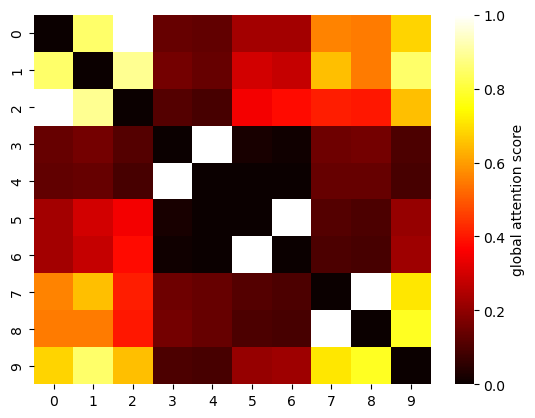
Global attention score heatmap (MF matrix)

Global attention score heatmap
Model MAE
Null (no edges) 0.397
Complete (45 edges) 0.088
Pruned (9 edges) 0.072
Oracle (8 edges) 0.070

18% lower MAE than complete graph

Ablation: Partial Interaction Groups (avg MAE, 10 runs)

$$y = \frac{1}{1+x_{0}^{2}+x_{1}^{2}+x_{2}^{2}} + \sqrt{\exp{(x_3+x_4)}} + |x₅+x₆| + x₇x₈x₉$$

Included groups MAE
{x₃,x₄}, {x₅,x₆}, {x₇,x₈,x₉} 0.079
{x₀,x₁,x₂}, {x₃,x₄}, {x₇,x₈,x₉} 0.091
{x₅,x₆}, {x₇,x₈,x₉} 0.101
{x₀,x₁,x₂}, {x₇,x₈,x₉} 0.117
{x₀,x₁,x₂}, {x₃,x₄}, {x₅,x₆} 0.155
9

Visual Comparison

Complete vs Ground Truth vs Learned Structure

Complete Graph

45 edges — all C(10,2) pairs

x₀ x₁ x₂ x₃ x₄ x₅ x₆ x₇ x₈ x₉ G₁ G₂ G₃ G₄

Ground Truth

8 edges — 4 interaction groups

x₀ x₁ x₂ x₃ x₄ x₅ x₆ x₇ x₈ x₉ G₁ G₂ G₃ G₄

Learned (Pruned)

9 edges (8 true + 1 FP)

FP: (x₁,x₉) x₀ x₁ x₂ x₃ x₄ x₅ x₆ x₇ x₈ x₉ G₁ G₂ G₃ G₄

✓ All 8 true edges recovered + 1 false positive

Learned graph closely mirrors ground truth structure

10

Discussion Insights

Why the method works and what the results tell us

Why Pruning Improves Accuracy

The complete graph exposes all pairwise channels, including many weak or noisy edges. Pruning removes them, reducing variance in message passing and simplifying the hypothesis space. Result: MAE 0.072 vs. 0.088 (complete).

Attention Heatmap Reveals Groups

The MF heatmap shows clear bright blocks at {x₀,x₁,x₂}, {x₃,x₄}, {x₅,x₆}, {x₇,x₈,x₉}—recovering the true group structure from attention alone. Dense within-group connectivity emerged without explicit higher-order operators.

Spurious Edges Are Infrequent

One spurious edge {x₁,x₉} appeared in the recovered set. Features can co-vary under the generative process or share downstream effects during training. Precision 0.89 confirms such false positives are rare.

Complexity vs Fit Trade-off

Edges MAE Null Complete Pruned Oracle

Important: This theoretical context motivates the work, but the core contribution is the empirical demonstration that attention-guided pruning recovers meaningful structure.

11

Limitations

Honest assessment of the controlled study

⚠️ Single Synthetic Dataset

Validated on one controlled dataset only. Real-world tabular/CTR datasets with unknown ground truth are needed before making broad generalizability claims.

⚠️ Model-Dependent Attention Scores

Attention scores are specific to TransformerConv. Different architectures may score edges differently; weak interaction effects may not surface in the attention signal.

⚠️ Spurious Edges Possible

One false edge {x₁,x₉} appeared—features co-varying under the generative process can inflate attention scores. Precision is 0.89, not 1.0.

⚠️ Threshold Needs Ground Truth

τ is selected by maximizing edge-level F₁ against known interaction pairs. No automatic threshold selection strategy for real-world settings (no ground truth) is yet proposed.

Scope of Validation

✓ Synthetic (validated) Real-world (future) Scalability (future)
12

Future Directions

Next steps for broader impact

Stability Selection Without Ground Truth

Replace the ground-truth threshold with data-driven stability selection, enabling reliable edge pruning on real-world datasets where oracle labels are unavailable.

🔗

Structural Priors & Regularizers

Combine attention scores with structural priors (e.g., sparsity regularization, domain constraints) to bias the discovered graph toward known interaction patterns.

Higher-Order (Hyperedge) Scoring

Extend MF scoring to explicitly model hyperedges, directly capturing three-way or k-way interactions instead of approximating them through pairwise proxy edges.

📊

Scaling & Real-World Benchmarks

Conduct scaling studies for larger feature dimensions and noisier regimes; benchmark on tabular and CTR datasets to validate generalization beyond the synthetic setting.

13

Conclusion

Key Takeaway

A simple global threshold on an attention-derived score (MF) recovers most true interaction edges (Precision 0.89, Recall 1.00, F₁=0.94) and creates a compact graph (9 vs. 45 edges) with lower prediction error than the complete graph.

✓ Method

Score–Prune–Retrain: one-layer TransformerConv → symmetrized MF score → global threshold τ → retrain from scratch on pruned graph.

✓ Results

9 edges recovered vs. 45 (complete) and 8 (oracle). MAE 0.072 (pruned) vs. 0.088 (complete) vs. 0.070 (oracle) vs. 0.397 (null).

✓ Insight

Removing noisy edges reduces message-passing variance. Pairwise attention proxies suffice to recover higher-order group structure in this controlled setting.

Thank You

Questions?

Phaphontee Yamchote

Advisor: Asst. Prof. Thanapon Noraset, Ph.D.

Co-advisor: Chainarong Amornbunchornvej, Ph.D.